深度学习基础入门与

PyTorch官方文档：docs.pytorch.org/docs/stable

1 基础知识

补充机器学习篇未着重讲的内容。

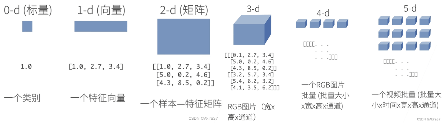
1.1 n阶张量

相关阅读：深度学习PyTorch代码模板

n维数组/n阶张量是机器学习和神经网络的主要数据结构

初始化：

x = torch.arange(10)        # tensor([0,  1,  2,  3,  4,  5,  6,  7,  8,  9])
x = torch.zeros((2, 3, 4))  # 全0
x = torch.ones((2, 3, 4))   # 全1
x = torch.randn(3, 4)       # 均值为0、标准差为1的标准正态分布
x = torch.tensor([[2, 1, 4, 3], [1, 2, 3, 4], [4, 3, 2, 1]])    # 根据(嵌套)列表为每个元素赋确定值

# 查看形状
x.shape     # 返回形状类：torch.Size(维度张量)
x.shape[0]  # 获取维度张量

# 获取元素个数
x.numel()   # 计算张量中元素的总数（维度的乘积）

# 变形
X = x.reshape(3, -1)    # 用-1自动计算维度

访问元素：

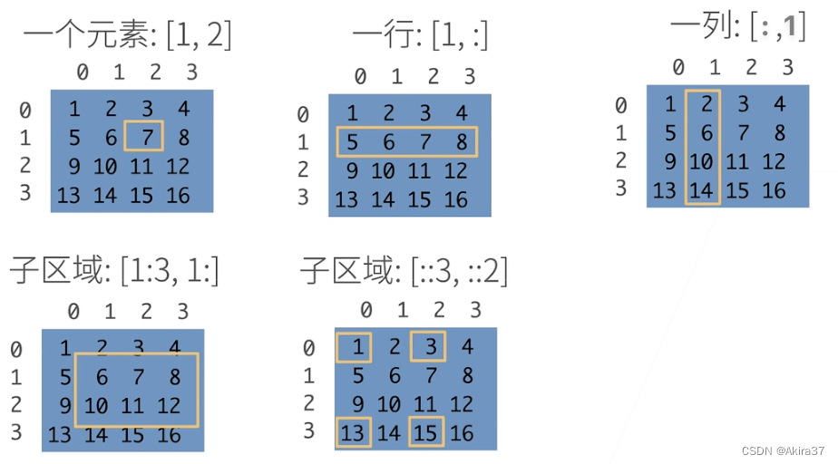
X[-1]       # 选择最后一个元素
X[1:3]      # 选择索引在[1, 3)上的元素（左开右闭，右-左 为切片长度，下同）

X[1, 2] = 9     # 指定索引写入元素
X[0:2, :] = 12  # 在索引0~1行批量写入元素

运算：

# 按元素运算
X + Y, X - Y, X * Y, X / Y, X ** Y      # 所有基本运算符均升级为按元素运算（形状不同则广播，下同）
torch.exp(X)    # 指数运算
X == Y          # 通过逻辑运算符构建二元张量（True / False）

# 连结（dim=x： 沿轴x……）
torch.cat((X, Y), dim=0)    # 沿轴0（行）连结张量（上下拼接）
torch.cat((X, Y), dim=1)    # 沿轴1（列）连结张量（左右拼接）

# 降维函数（详见下文）
X.sum()     # 求和（返回只含1个元素的张量，下同）
X.mean()    # 求平均值

# 与NumPy数组的转换
A = X.numpy()           # 张量转化为n维数组（numpy.ndarray）
B = torch.tensor(A)     # n维数组转化为张量（torch.Tensor）

# 与Python标量的转换
a = torch.tensor([3.7]) # 大小为1的张量 tensor([3.7000])
a.item()                # 调用方法获取元素
float(a), int(a)        # 使用python

1.2 数据预处理

相关阅读：数据分析与应用

创建人工数据集：随机生成一个人工数据集，存储于csv（逗号分割值）文件中

import os

os.makedirs(os.path.join('..', 'data'), exist_ok=True)
data_file = os.path.join('..', 'data', 'house_tiny.csv')
with open(data_file, 'w') as f:
    f.write('NumRooms, Alley, Price\n')       # 列名
    f.write('NA, Pave, 127500\n')         # 每行表示一个数据样本
    f.write('2, NA, 106000\n')
    f.write('4, NA, 178100\n')
    f.write('NA, NA, 140000\n')

读取数据集：从创建的csv文件中加载原始数据集

import pandas as pd

data = pd.read_csv(data_file)   # pandas读取csv文件
print(data)

处理缺失数据：

# 使用插值法
inputs, outputs = data.iloc[:, 0:2], data.iloc[:, 2]
inputs = inputs.fillna(inputs.mean())           # 填充缺失值为均值（仅适用于数值类型数据）
inputs = pd.get_dummies(inputs, dummy_na=True)  # 视为特征：缺失值 - Alley_nan，Str - Alley

# 所有条目都是数值类型，故可转换成张量
X, y = torch.tensor(inputs.values), torch.tensor(outputs.values)

1.3 线性代数

相关阅读：线性代数（数二强化冲刺笔记）

标量

按元素操作：

\begin{aligned}
c&=a+b\\
c &=a\cdot b\\
c &=\sin a
\end{aligned}

长度：

\begin{aligned}
|a|&=\begin{cases}
 a, & a>0 \\
 -a, & \text{otherwise}
\end{cases}\\
|a+b|&≤|a|+|b|\\
|a \cdot b| &=|a| \cdot |b|
\end{aligned}

向量

按元素操作：

\begin{aligned}
\mathbf{c} &=\mathbf{a}+\mathbf{b}\ \text{ where }\ c_i=a_i+b_i\\
\mathbf{c} &=a \cdot \mathbf{b}\ \text{ where }\ c_i=a\cdot b_i\\
\mathbf{c} &=\sin \mathbf{a}\ \text{ where }\ c_i=\sin a_i
\end{aligned}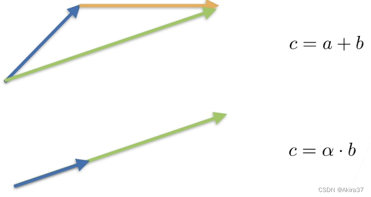

长度（L_2范数）：

\begin{aligned}
\left\| \mathbf{a}\right\| &=\left (\sum\limits_{i} a_i^2\right)^{\frac12}≥0\\
\left\| a \cdot \mathbf{b} \right\| &=|a| \cdot \left\| \mathbf{b}\right\|
\end{aligned}

点积：

\begin{aligned}
\left \langle \mathbf{a},\mathbf{b} \right \rangle &=\mathbf{a}^{\text{T}}\mathbf{b}=\sum_i a_ib_i \\ \left \langle \mathbf{a},\mathbf{b} \right \rangle &=0 \Leftrightarrow \mathbf{a}\ \bot\ \mathbf{b}
\end{aligned}

矩阵

按元素操作：

\begin{aligned}
\mathbf{C} &=\mathbf{A}+\mathbf{B}\ \text{ where }\ C_{ij}=A_{ij}+B_{ij}\\
\mathbf{C} &=a \mathbf{B}\ \text{ where }\ C_{ij}=a B_{ij}\\
\mathbf{C} &=\sin \mathbf{A}\ \text{ where }\ C_{ij}=\sin A_{ij}
\end{aligned}

矩阵向量积：

\begin{aligned}
\mathbf{c}&=\mathbf{Ab}\ \text{ where }\ c_i=\sum\limits_j A_{ij}b_j
\end{aligned}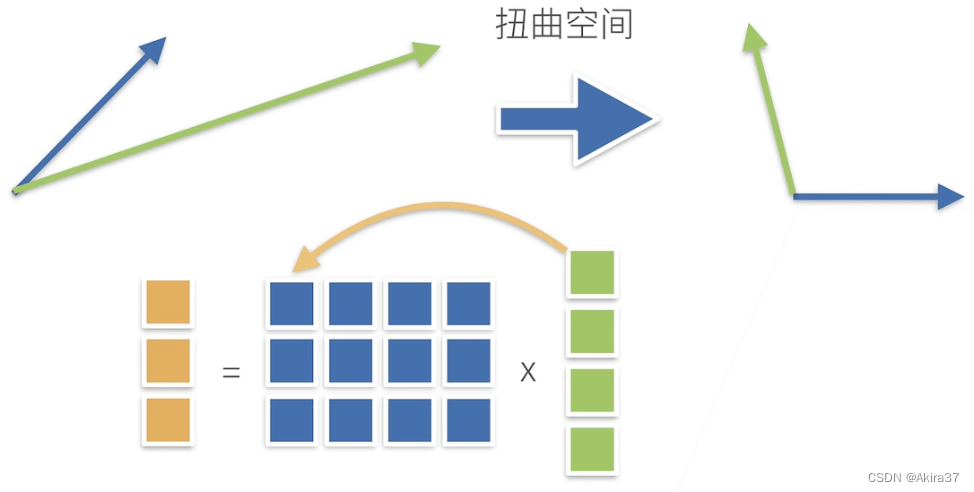

矩阵乘法：

\begin{aligned}
\mathbf{C}=\mathbf{AB}\ \text{ where }\ C_{ik}=\sum_j A_{ij}B_{jk}
\end{aligned}

范数：

• 矩阵范数（存在多种具体定义，暂略） ：在满足向量范数各条件的基础上，还满足以下条件

\begin{aligned}
\mathbf{c}&=\mathbf{Ab}\ \text{ hence } \left\| \mathbf{c}\right\|≤\left\|\mathbf{A}\right\|\cdot\left\| \mathbf{b}\right\|
\end{aligned}

• Frobenius范数（更常用）

\begin{aligned}
\left\| \mathbf{A}\right\|_{\text{Frob}}=\left (\sum\limits_{i}\sum\limits_{j}A_{ij}^2\right)^{\frac12}
\end{aligned}

特殊矩阵：

• 对称矩阵、反对称矩阵：A_{ij}=A_{ji}、A_{ij}=-A_{ji}
• 正定矩阵：

\begin{aligned}
\left\| \mathbf{x}\right\|^2=\mathbf{x}^{\text{T}}\mathbf{x}≥0\ \text{ generalizes to }\ \mathbf{x}^{\text{T}}\mathbf{Ax}≥0
\end{aligned}

• 正交矩阵：\mathbf{Q}\mathbf{Q}^\top=\mathbf{I}
• 置换矩阵（置换矩阵必正交）：

\begin{aligned}
\mathbf{P}\ \text{ where }\ P_{ij}=1\ \text{ if and only if }\ j=\pi(i)
\end{aligned}

• 特征向量（不被矩阵改变方向）和特征值：\mathbf{Ax}=\lambda \mathbf{x}

PyTorch实现

a = torch.tensor([3.0])
x = torch.arange(10, dtype=torch.float32)
A = torch.arange(20, dtype=torch.float32).reshape(5, 4) # 5x4的矩阵

len(x)
A.shape

# 转置
A.T

# 深拷贝
B = A.clone()

# 按元素操作
A + B
A * B   # 哈达玛积

# 求和
A.sum()             # 对所有元素求和，降为标量
A.sum(axis=0)       # 沿轴0（行）求和，降为向量（参考连结方法cat()）
A.sum(axis=[0, 1])  # 沿轴0、轴1求和，同方法sum()
# 求平均值
A.mean()            # 等价于 A.sum() / A.numel() 
A.mean(axis=0)      # 等价于 A.sum(axis=0) / A.shape[0]
# 保持轴数不变，便于广播
sum_A = A.sum(axis=1, keepdims=True)    # 对每一行求和
A / sum_A           # 每个元素分别除以其所在行元素和
# 累加求和
A.cumsum(axis=0)    # 沿轴0累加求和（形状不变）

# 向量点积（PyTorch的点积只能计算向量！）
torch.dot(x, y)     # 等价于torch.sum(x * y)

# 矩阵向量积
torch.mv(A, x)

# 矩阵乘法
torch.mm(A, A)

# L2范数：向量元素的平方和的平方根
torch.norm(x)
# L1范数：向量元素的绝对值之和
torch.abs(x).sum()
# Frobenius范数：矩阵元素的平方和的平方根
torch.norm(A)

1.4 梯度

梯度（gradient）是一个向量，指向函数变化率最大的方向。

\begin{array}{c|lll}\\
 &\begin{aligned}x\in \mathbb{R}\end{aligned} & \begin{aligned}\mathbf{x} \in \mathbb{R}^{n}\end{aligned} & \begin{aligned}\mathbf{X}\in \mathbb{R}^{n\times k}\end{aligned}\\
\hline\\
\begin{aligned}y\in \mathbb{R}\end{aligned}  & \begin{aligned}\frac{\partial y}{\partial x}\in \mathbb{R}\end{aligned}  & \begin{aligned}\frac{\partial y}{\partial \mathbf{x}}\in \mathbb{R}^{1\times n}\end{aligned} & \begin{aligned}\frac{\partial y}{\partial \mathbf{X}} \in \mathbb{R}^{k\times n}\end{aligned} \\
\begin{aligned}\mathbf{y}\in \mathbb{R}^{m}\end{aligned}  & \begin{aligned}\frac{\partial \mathbf{y}}{\partial x} \in \mathbb{R}^{m}\end{aligned}  & \begin{aligned}\frac{\partial \mathbf{y} }{\partial \mathbf{x} }\in \mathbb{R}^{m\times n}\end{aligned} & \begin{aligned}\frac{\partial \mathbf{y}}{\partial \mathbf{X}} \in \mathbb{R}^{m\times n\times k}\end{aligned}  \\
\begin{aligned}\mathbf{Y} \in \mathbb{R}^{m\times l}\end{aligned} & \begin{aligned}\frac{\partial \mathbf{Y}}{\partial x} \in \mathbb{R}^{m\times l}\end{aligned}  & \begin{aligned}\frac{\partial \mathbf{Y}}{\partial \mathbf{x}} \in \mathbb{R}^{m\times l\times n}\end{aligned}  & \begin{aligned}\frac{\partial \mathbf{Y}}{\partial \mathbf{X}} \in \mathbb{R}^{m\times l\times k\times n}\end{aligned}\\
\\\end{array}

标量导数

对于单变量函数，梯度即为导数\frac{\text{d}y}{\text{d}x}

\begin{array}{c|llllllll}\\
\begin{aligned}y\end{aligned} & \begin{aligned}a\end{aligned} & \begin{aligned}x^n\end{aligned} & \begin{aligned}\exp(x)\end{aligned} & \begin{aligned}\log x\end{aligned} & \begin{aligned}\sin x\end{aligned} & \begin{aligned}u+v\end{aligned} & \begin{aligned}uv\end{aligned} & \begin{aligned}u(x)\end{aligned}\\
\\\hline\\
\begin{aligned}\frac{\text{d}y}{\text{d}x}\end{aligned} & \begin{aligned}0\end{aligned} & \begin{aligned}nx^{n-1}\end{aligned} & \begin{aligned}\exp(x)\end{aligned} & \begin{aligned}\frac1x\end{aligned} & \begin{aligned}\cos x\end{aligned} & \begin{aligned}\frac{\text{d}u}{\text{d}x}+\frac{\text{d}v}{\text{d}x}\end{aligned} & \begin{aligned}\frac{\text{d}u}{\text{d}x}v+\frac{\text{d}v}{\text{d}x}u\end{aligned} & \begin{aligned}\frac{\text{d}y}{\text{d}u}\frac{\text{d}u}{\text{d}x}\end{aligned}\\
\\\end{array}

标量对向量求导

标量y对向量\mathbf{x}的每一个分量求导，组成行向量

\begin{aligned}
\mathbf{x}&=(x_1,x_2,\dots,x_n)^\top\\
\frac{\partial y}{\partial \mathbf{x} } &=\left(
 \frac{\partial y}{\partial x_1} , \frac{\partial y}{\partial x_2} ,\dots, \frac{\partial y}{\partial x_n}\right)
 \end{aligned}

\begin{array}{c|llllllll}\\
\begin{aligned}y\end{aligned} & \begin{aligned}a\end{aligned} & \begin{aligned}\text{sum}(\mathbf{x})\end{aligned} & \begin{aligned}\lVert \mathbf{x}  \rVert^2\end{aligned} & \begin{aligned}au\end{aligned} & \begin{aligned}u+v\end{aligned} & \begin{aligned}uv\end{aligned} & \begin{aligned}\left \langle \mathbf{u} ,\mathbf{v}  \right \rangle\end{aligned}\\
\\\hline\\
\begin{aligned}\frac{\partial y}{\partial \mathbf{x} }\end{aligned} & \begin{aligned}\mathbf{0}^\top\end{aligned}  & \begin{aligned}\mathbf{1}^{\top}\end{aligned} & \begin{aligned}2\mathbf{x}^\top\end{aligned} & \begin{aligned}a\frac{\partial u}{\partial \mathbf{x} }\end{aligned} & \begin{aligned}\frac{\partial u}{\partial \mathbf{x}}+\frac{\partial v}{\partial \mathbf{x}}\end{aligned} & \begin{aligned}\frac{\partial u}{\partial \mathbf{x}}v+\frac{\partial v}{\partial \mathbf{x}}u\end{aligned} & \begin{aligned}\mathbf{u}^{\top}\frac{\partial \mathbf{v}}{\partial \mathbf{x}}+\mathbf{v}^{\top}\frac{\partial \mathbf{u}}{\partial \mathbf{x}}\end{aligned} & 
\\ \\\end{array}

向量对标量求导

向量\mathbf{y}的每一个分量对标量x求导，组成列向量

\begin{aligned}
\mathbf{y}=\left(\begin{matrix}
y_1 \\
y_2 \\
\vdots \\
y_m
\end{matrix}\right),\ 
\frac{\partial \mathbf{y}}{\partial x} =\left(\begin{matrix}
\frac{\partial y_1}{\partial x} \\
\frac{\partial y_1}{\partial x} \\
\vdots \\
\frac{\partial y_m}{\partial x}
\end{matrix}\right)
\end{aligned}

向量对向量求导

向量\mathbf{y}的每一个分量对向量\mathbf{x}的每一个分量求导，先展开\mathbf{y}再展开\mathbf{x}可得，结果为矩阵

\begin{aligned}
\mathbf{x}=\left(\begin{matrix}
x_1 \\
x_2 \\
\vdots \\
x_n
\end{matrix}\right),\ \mathbf{y}=\left(\begin{matrix}
y_1 \\
y_2 \\
\vdots \\
y_m
\end{matrix}\right),\ 
\frac{\partial \mathbf{y} }{\partial \mathbf{x} }=\left(\begin{matrix}
\frac{\partial y_1}{\partial \mathbf{x} }  \\
\frac{\partial y_2}{\partial \mathbf{x} } \\
\vdots \\
\frac{\partial y_m}{\partial \mathbf{x} }
\end{matrix}\right)
=\left(\begin{matrix}
\frac{\partial y_1}{\partial x_1}&\frac{\partial y_1}{\partial x_2}&\cdots&\frac{\partial y_1}{\partial x_n}  \\
\frac{\partial y_2}{\partial x_1}&\frac{\partial y_2}{\partial x_2}&\cdots&\frac{\partial y_2}{\partial x_n} \\
\vdots&\vdots&&\vdots \\
\frac{\partial y_m}{\partial x_1}&\frac{\partial y_m}{\partial x_2}&\cdots&\frac{\partial y_m}{\partial x_n}
\end{matrix}\right)
\end{aligned}

\begin{array}{c|llllllll}\\
\mathbf{y} & \mathbf{a} & \mathbf{x} & \mathbf{Ax} & \mathbf{x}^{\top}\mathbf{A} & a\mathbf{u} & \mathbf{Au} & \mathbf{u}+\mathbf{v}\\
\\\hline\\
\frac{\partial \mathbf{y} }{\partial \mathbf{x} } & \mathbf{0} & \mathbf{I} & \mathbf{A} & \mathbf{A}^{\top} & a\frac{\partial \mathbf{u} }{\partial \mathbf{x} } & \mathbf{A}\frac{\partial \mathbf{u} }{\partial \mathbf{x} } & \frac{\partial \mathbf{u} }{\partial \mathbf{x} }+\frac{\partial \mathbf{v} }{\partial \mathbf{x} }
\\ \\\end{array}

1.5 自动微分

相关阅读：高等数学（数二强化冲刺笔记）

向量链式法则

将标量链式法则拓展到向量，可得

\begin{aligned}
\underset{(1,n)}{\frac{\partial y}{\partial \mathbf{x}}}=\underset{(1,)}{\frac{\partial y}{\partial u}}\underset{(1,n)}{\frac{\partial u}{\partial \mathbf{x} }},\ 
\underset{(1,n)}{\frac{\partial y}{\partial \mathbf{x} }}=\underset{(1,k)}{\frac{\partial y}{\partial \mathbf{u} }}\underset{(k,n)}{\frac{\partial \mathbf{u} }{\partial \mathbf{x} }},\ 
\underset{(m,n)}{\frac{\partial \mathbf{y} }{\partial \mathbf{x} }}=\underset{(m,k)}{\frac{\partial \mathbf{y} }{\partial \mathbf{u} }}\underset{(k,n)}{\frac{\partial \mathbf{u} }{\partial \mathbf{x}}}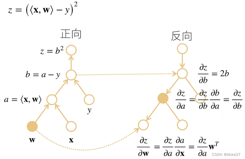
\end{aligned}

【例1】设\mathbf{x},\mathbf{w} \in \mathbb{R}^n,\ y\in \mathbb{R},\ z=\left(\left \langle \mathbf{x},\mathbf{w} \right \rangle -y \right)^2，求 \frac{\partial z}{\partial \mathbf{w} }

【解】令 a=\left \langle \mathbf{x},\mathbf{w} \right \rangle,\ b=a-y,\ z=b^2 ，则

\begin{aligned}
\frac{\partial z}{\partial \mathbf{w} } &=\frac{\partial z}{\partial b} \frac{\partial b}{\partial a} \frac{\partial a}{\partial \mathbf{w} }\\
& =\frac{\partial b^2}{\partial b}\frac{\partial (a-y)}{\partial a}\frac{\partial \left \langle \mathbf{x},\mathbf{w} \right \rangle}{\partial \mathbf{w}}\\
&=  2b \cdot1\cdot \mathbf{x}^{\top}\\
 &=  2\left(\left \langle \mathbf{x},\mathbf{w} \right \rangle -y\right) \mathbf{x}^{\top}
\end{aligned}

【例2】设\mathbf{X} \in \mathbb{R}^{m\times n},\ \mathbf{w} \in \mathbb{R}^n,\ \mathbf{y}\in \mathbb{R}^m,\ z=\lVert\mathbf{Xw}-\mathbf{y} \rVert^2，求\frac{\partial z}{\partial \mathbf{w} }

【解】令\mathbf{a}=\mathbf{Xw},\ \mathbf{b}=\mathbf{a}-\mathbf{y},\ z=\lVert \mathbf{b} \rVert^2，则

\begin{aligned}
\frac{\partial z}{\partial \mathbf{w} } &=  \frac{\partial z}{\partial \mathbf{b} } \frac{\partial \mathbf{b} }{\partial \mathbf{a} } \frac{\partial \mathbf{a} }{\partial \mathbf{w} }\\
 &= \frac{\partial \lVert\mathbf{b}\rVert ^2}{\partial \mathbf{b} }\frac{\partial (\mathbf{a}-\mathbf{y})}{\partial \mathbf{a} }\frac{\partial (\mathbf{Xw})}{\partial \mathbf{w}}\\
&= 2\mathbf{b}^{\top}  \times\mathbf{I} \times \mathbf{X}\\
&= 2(\mathbf{Xw} -\mathbf{y} )^{\top}\mathbf{X}
\end{aligned}

自动求导

自动求导计算一个函数在指定值上的导数：1. 将代码分解成操作子；2. 将计算表示成一个无环图（计算图）

符号求导：\frac{\text{d}}{\text{d}x}(4x^3 + x^2 + 3)=12x^2 +2x

数值求导：\frac{\text{d} f(x)}{\text{d} x} =\lim\limits_{h \to 0} \frac{f(x+h)-f(x)}{h}

由链式法则\frac{\partial y}{\partial x}=\frac{\partial y}{\partial u_n}\frac{\partial u_n}{\partial u_{n-1}}\cdots\frac{\partial u_2}{\partial u_1}\frac{\partial u_1}{\partial x}可得自动求导的两种模式：

1. 正向累积（时间复杂度太高，不适合自动求导）：

   \begin{aligned}
   \frac{\partial y}{\partial x}=\frac{\partial y}{\partial u_n}\left(\frac{\partial u_n}{\partial u_{n-1}}\left(\cdots\left(\frac{\partial u_2}{\partial u_1}\frac{\partial u_1}{\partial x}\right)\right)\right)
   \end{aligned}

2. 反向累积（反向传递）：

\begin{aligned}
\frac{\partial y}{\partial x}=\left(\left(\left(\frac{\partial y}{\partial u_n}\frac{\partial u_n}{\partial u_{n-1}}\right)\cdots\right)\frac{\partial u_2}{\partial u_1}\right)\frac{\partial u_1}{\partial x}
\end{aligned}

反向传递的过程：

1. 构造计算图
2. 前向：执行图，存储中间结果
3. 反向：从反方向执行图（同时去除不需要的枝）

【例】如下所示的计算图描述了前馈和反馈的流程

PyTorch实现

【例1】设函数y=2\mathbf{x}^{\text{T}}\mathbf{x} ，通过自动求导求\frac{\partial y}{\partial \mathbf{x} }

import torch

# x = torch.arange(4.0)     # tensor([0., 1., 2., 3.])
x = torch.arange(4.0, requires_grad=True)   # 开启梯度存储，用x.grad获取梯度
y = 2 * torch.dot(x, x)     # tensor(28., grad_fn=<MulBackward0>)
y.backward()    # 调用反向传播函数来自动计算标量y关于向量x每个分量的梯度

x.grad  # (tensor([0., 4., 8., 12.])

【例2】设函数y=\text{sum}(\mathbf{x})，通过自动求导求\frac{\partial y}{\partial \mathbf{x} }

x.grad.zero_()  # PyTorch默认累积梯度，故需清除之前的梯度（以单下划线结尾的函数表示重写内容）
y = x.sum()
y.backward()

x.grad  # tensor([1., 1., 1., 1.])

【例3】设函数\mathbf{y}=\mathbf{x}\odot \mathbf{x}，通过自动求导求\frac{\partial \mathbf{y}}{\partial \mathbf{x} }

深度学习中目的不是计算微分矩阵，而是批量中每个样本单独计算的偏导数之和。

对非标量调用backward()需要传入一个gradient参数，该参数指定微分函数关于self的梯度
本例只想求偏导数的和，所以应传入分量全为1的梯度（由求导公式\frac{\partial \text{sum}(\mathbf{x} )}{\partial \mathbf{x} } =\mathbf{1}^{\text{T} }可得）

x.grad_zero_()
y = x * x
y.sum().backward()  # 等价于 y.backward(torch.ones(len(x)))

x.grad  # tensor([0., 2., 4., 6.])

【例4】构建如下函数的计算图需经过Python控制流，计算变量的梯度

def f(a):
    b = a * 2
    while b.norm() < 1000:
        b *= 2
    if b.sum() > 0:
        c = b
    else:
        c = 100 * b
    return c

a = torch.randn(size=(), requires_grad=True)
d = f(a)    # d实为关于a的线性函数，因此梯度即为该直线的斜率
d.backward()

a.grad == d / a     # tensor(True)

1.6 概率

相关阅读：概率论与数理统计常用公式大全

简单回顾各种重要概念以及多个随机变量的运算。

基本概率论

抽样（Sampling）是统计学中把从概率分布中抽取样本的过程。分布（Distribution）可以视为对事件（Event）的概率分配，将概率分配给一些离散选择的分布称为多项分布（Multinomial Distribution）。随机变量（Random Variable）可以在随机实验的一组可能性中取一个值。

事件（Event）是一组给定样本空间（Sample Space，或称结果空间，Outcome Space）的随机结果。若对于所有i≠j都有\mathcal{A}_i \cap \mathcal{A}_j=\emptyset，则称这两个事件互斥（Mutually Exclusive）。

概率（Probability）可以被认为是将集合映射到真实值的函数。在给定的样本空间\mathcal{S}中，事件\mathcal{A}的概率表示为P(\mathcal{A})。概率满足以下3条概率论公理：

1. 对于任意事件\mathcal{A}，其概率必定非负，即P(\mathcal{A})≥0
2. 整个样本空间的概率为1，即P(\mathcal{S})=1
3. 对于互斥事件的任一可数序列\mathcal{A}_1,\mathcal{A}_2,\cdots，序列中任意一个事件发生的概率等于它们各自发生的概率之和，即P(\bigcup\limits_{i=1}^{\infin} \mathcal{A}_i)=\sum\limits_{i=1}^{\infin} P(\mathcal{A}_i)

联合概率

联合概率（Joint Probability）P(A=a,B=b)表示同时满足A=a和B=b的概率，对于任意a,b，有

\begin{aligned}
P(A=a,B=b)≤\min\{P(A=a),P(B=b)\}
\end{aligned}

条件概率

由联合概率的不等式可得0≤\frac{P(A=a,B=b)}{P(A=a)}≤1。将上式中的比率称为条件概率（Conditional Probability），记为P(B=b \mid A=a)，即

\begin{aligned}
P(B=b \mid A=a)=\frac{P(A=a,B=b)}{P(A=a)}
\end{aligned}

贝叶斯定理

Bayes定理（Bayes’ Theorem）：根据乘法法则（multiplication rule ）可得P(A,B)=P(B\mid A)P(A)，根据对称性可得P(A,B)=P(A\mid B)P(B)，设P(B)>0，则有

\begin{aligned}
P(A\mid B)=\frac{P(B\mid A)P(A)}{P(B)}
\end{aligned}

求和法则

求和法则（Sum Rule）：求 $B$ 的概率相当于计算A的所有可能选择，并将所有选择的联合概率聚合在一起，即

\begin{aligned}
P(B)=\sum\limits_A P(A,B)
\end{aligned}

该操作又称为边际化（Marginalization），边际化结果的概率或分布称为边际概率（Marginal Probability） 或边际分布（Marginal Distribution）。

独立性

如果事件A的发生跟事件 $B$ 的发生无关，则称两个随机变量A和B是独立（Dependence）的，记为

\begin{aligned}
A \perp  B
 \end{aligned}

易得此时P(A\mid B)=P(A)。在所有其他情况下，称A和B依赖（Independence）。

同理，若对于三个随机变量A,B,C有P(A,B\mid C)=P(A\mid C)P(B\mid C)，则称A和B是条件独立（Conditionally Independent）的，记为

\begin{aligned}
A \perp  B \mid C
 \end{aligned}

期望和方差

为了概括概率分布的关键特征，需要一些测量方法。

一个随机变量X的期望（expectation，或平均值，Average）表示为

\begin{aligned}
E[X]=\sum\limits_x xP(X=x)
\end{aligned}

当函数f(x)的输入是从分布P中抽取的随机变量时，f(x)的期望值为

\begin{aligned}
E_{x\sim P}[f(x)]=\sum_xf(x)P(x)
\end{aligned}

方差（Variance）可以量化随机变量与其期望值的偏置，定义为

\begin{aligned}
\text{Var}[X]=E[(X-E[X])^2]=E[X^2]-E^2[X]
\end{aligned}

方差的平方根称为标准差（Standard Deviation）。
随机变量函数f(x)的方差衡量的是：当从该随机变量分布中采样不同值x时， 函数值偏离该函数的期望的程度，即

\begin{aligned}
\text{Var}[f(x)]=E[(f(x)-E[f(x)])^2]
\end{aligned}

1.A 如何读论文

1. Title
2. Abstract
3. Introduction
4. Method
5. Experiments
6. Conclusion

第一遍：标题、摘要、结论。可以看一看方法和实验部分重要的图和表。这样可以花费十几分钟时间了解到论文是否适合你的研究方向。

第二遍：确定论文值得读之后，可以快速的把整个论文过一遍，不需要知道所有的细节，需要了解重要的图和表，知道每一个部分在干什么，圈出相关文献。觉得文章太难，可以读引用的文献。

第三遍：提出什么问题，用什么方法来解决这个问题。实验是怎么做的。合上文章，回忆每一个部分在讲什么。

---

2 线性回归

线性回归（Linear Regression）是对n维输入的加权，外加偏差，可视为单层神经网络。

2.1 多元线性回归

给定n维特征输入\mathbf{x}^{(i)} =(x_1,x_2,\dots,x_n)^\top，n维权重\mathbf{w} =(w_1,w_2,\dots,w_n)^\top，标量偏差b，则预测值为

\begin{aligned}
\hat y^{(i)} =\mathbf{w}^\top\mathbf{x}^{(i)} +b
\end{aligned}

对于有多个样本的特征集合\mathbf{X}，对应的预测值集合为

\begin{aligned}
\mathbf{\hat y}=\mathbf{X}\mathbf{w}+b
\end{aligned}

net = nn.Sequential(nn.Linear(2, 1))

net[0].weight.data.normal_(0, 0.01)
net[0].bias.data.fill_(0)

2.2 回归损失函数：均方误差（L2损失）

损失函数（Loss Function）能够量化目标的实际值与预测值之间的差距。 通常选择非负数作为损失，且数值越小表示损失越小，完美预测时的损失为0。

均方误差/L2损失（Mean Square Error，MSE，L2 Loss）是回归问题中最常用的损失函数。当样本i的预测值为\hat y^{(i)}，其相应的真实标签为y^{(i)}，则其平方误差为

\begin{aligned}
l^{(i)}(\mathbf{w},b)=\frac12(\hat y^{(i)}-y^{(i)})^2
\end{aligned}

为了度量模型在整个数据集上的质量，需计算在训练集n个样本上的损失均值，即可得均方误差

\begin{aligned}
L(\mathbf{w},b) &=\frac1n\sum\limits_{i=1}^n l^{(i)}(\mathbf{w},b)\\
&=\frac1n\sum\limits_{i=1}^n\frac12(\mathbf{w}^\top\mathbf{x}^{(i)}+b-y^{(i)})^2\\
&=\frac1{2n}\lVert \mathbf{Xw}+b-\mathbf{y}\rVert^2
\end{aligned}

最小化损失来学习参数

\begin{aligned}
(\mathbf{w}^*,b^*)=\argmin\limits_{(\mathbf{w},b)} L(\mathbf{w},b)
\end{aligned}

loss = nn.MSELoss()

3.3 解析解

线性回归的解可以用一个公式简单地表达出来， 这类解叫作解析解（Analytical Solution）或显示解。将偏置b合并到参数\mathbf{w}中，在包含所有参数的矩阵中附加一列，即

\begin{aligned}
\mathbf{X} &\gets \left(\mathbf{X},\mathbf{1}\right)\\
\mathbf{w} &\gets\left(\mathbf{w},b\right)^\top
\end{aligned}

则损失函数可化为L(\mathbf{w})=\frac1{2n}\lVert \mathbf{y}-\mathbf{Xw} \rVert^2，为凸函数，故最优解\mathbf{w}^*满足

\begin{aligned}
\frac{\partial L(\mathbf{w})}{\partial \mathbf{w} } &= \frac1n(\mathbf{y}-\mathbf{Xw})^\top\mathbf{X}=0\\
\mathbf{w}^* &=(\mathbf{X}^\text{T}\mathbf{X})^{-1}\mathbf{X}^\text{T}\mathbf{y} 
\end{aligned}

回归问题常用的求解方法——梯度下降（更多方法详见第5章）：

• 梯度下降（Gradient Descent）：初始化模型参数的值（如随机初始化），计算损失函数（损失均值）关于模型参数的导数（梯度），不断地在损失函数递减的方向上更新参数来降低误差，即

\begin{aligned}
(\mathbf{w},b )\leftarrow(\mathbf{w},b)-η\partial_{(\mathbf{w},b)}L(\mathbf{w},b)
\end{aligned}

• 小批量随机梯度下降（Minibatch Stochastic Gradient Descent）：为深度学习默认的求解方法。原始方法实际执行的效率可能会非常慢，因为在每一次更新参数之前须遍历整个数据集。因此在每次需要计算更新的时候随机抽取一个小批量\mathcal{B}，即

\begin{aligned}
(\mathbf{w},b )\leftarrow(\mathbf{w},b)-\frac{η}{\mathcal{|B|} }\sum\limits_{i\in |\mathcal{B}| }\partial_{(\mathbf{w},b)}l^{(i)}(\mathbf{w},b)
\end{aligned}

其中η为学习率（Learning Rate），|\mathcal{B}|为批量大小（Batch Size），这种手动预先指定而非训练时调整的参数称为超参数（Hyperparameter）。

# 设置参数和学习率
trainer = torch.optim.SGD(net.parameters(), lr=0.03)

---

3 Softmax回归

分类问题中更常用Softmax回归。

3.1 分类问题

回归（Regression）与分类（Classification）的区别：

• 回归估计一个连续值：
  1. 单连续数值输出
  2. 自然区间\mathbb{R}
  3. 跟真实值的区别作为损失
• 分类预测一个离散类别：
  1. 通常多个输出
  2. 输出i是预测为第i类的置信度

独热编码（One-hot Encoding）：是一个向量，分量和类别一样多， 类别对应的分量设置为1，其他所有分量设置为。假设真实类别为y，对类别进行一位有效编码，则独热编码为

\begin{aligned}
\mathbf{y}=(y_1,y_2,\dots,y_n)^\top\ ,\ y_i=\begin{cases}  1, &
i=y \\  0, & \text{otherwise} \end{cases}
\end{aligned}

3.2 Softmax运算

Softmax回归是另一种单层神经网络，用于处理多类分类问题，需要与未规范化的输出\mathbf{o}=(o_1,o_1,\dots,o_n)^\top数量相同的仿射函数（Affine Function），每个输出对应的仿射函数及其向量表示分别为

\begin{aligned}
o_i&=\sum_{j} x_jw_{ij}+b_i,\ i=1,2,\dots,n\\
\mathbf{o}&=\mathbf{Wx}+\mathbf{b}
\end{aligned}

使用Softmax函数得到每个类的预测置信度：将输出变换为非负数且总和为1，使得\mathbf{\hat y}=(\hat y_1,\hat y_2,\dots,\hat y_n)^\top中对于所有i都有0≤\hat y_i≤1，且\sum\limits_i y_i = 1，如下式

\begin{aligned}
\mathbf{\hat y}=\text{softmax}(\mathbf{o})\ \text{ where }\ \hat y_i=\frac{\exp(o_i)}{\sum\limits_k\exp(o_k)}
\end{aligned}

此时\mathbf{\hat y}可视为一个正确的概率分布，因此将具有最大输出值的类别作为预测值，即

\begin{aligned}
\hat y=\argmax_i \hat y_i=\argmax_i o_i
\end{aligned}

# PyTorch不会隐式地调整输入的形状，因此需在线性层前定义展平层来调整网络输入的形状
net = nn.Sequential(nn.Flatten(), nn.Linear(784, 10))   # softmax操作已整合进loss中

def init_weights(m):
    """初始化参数"""
    if type(m) == nn.Linear:    # 仅初始化全连接层
        nn.init.normal_(m.weight, std=0.01)

net.apply(init_weights)     # 对模型所有层操作

3.3 分类损失函数：交叉熵损失

交叉熵（Cross-entropy）是分类问题中常见的损失函数，可用于衡量两个概率的区别：

\begin{aligned}
H(\mathbf{p},\mathbf{q})=-\sum_i p_i\log q_i
\end{aligned}

分类问题常将真实概率\mathbf{y}和预测概率 \mathbf{\hat y}的区别作为损失，因此常用交叉熵损失函数，如下式

\begin{aligned}
l(\mathbf{y},\mathbf{\hat y})=-\sum_i y_i\log \hat y_i
\end{aligned}

# 该损失函数整合了softmax操作
loss = nn.CrossEntropyLoss()

交叉熵函数的梯度：利用softmax的定义，将上式变形、对未规范化的输出o_i求导得

\begin{aligned}
 l(\mathbf{y},\mathbf{\hat y}) &= -\sum_i y_i \log \frac{\exp(o_i)}{\sum\limits_k \exp(o_k)}\\
 &= \sum_i y_i \log \sum_k \exp(o_k) -\sum_i y_io_i \\
 &=  \log \sum_k\exp(o_k)-\sum_iy_io_i\\
\partial_{o_i}l(\mathbf{y},\mathbf{\hat y}) &=\frac{\exp(o_i)}{\sum\limits_k \exp(o_k)}-y_i\\
&=\text{softmax}(\mathbf{o})_i-y_i
\end{aligned}

其中\text{softmax}(\mathbf{o})_i表示预测\mathbf{\hat y}的第i个分量（即\hat y_i，见softmax定义式）。该梯度正为真实概率与预测概率的区别。

---

4 多层感知机

狭义上的深度神经网络指的就是MLP。

4.1 从感知机到MLP

感知机（Perceptron）是最早的AI模型之一。给定输入\mathbf{x}、权重\mathbf{w}、偏移b，感知机输出

\begin{aligned}
o=\sigma(\mathbf{w}^\top\mathbf{x} +b),\ \sigma(x)=\begin{cases}  1, & x>0 \\  -1, &
\text{otherwise}  \end{cases}
\end{aligned}

输出为二分类，求解算法等价于使用批量大小为1的梯度下降。不能拟合XOR函数。

多层感知机（Multilayer Perceptron, MLP）在网络中加入一定层数的隐藏层（Hidden Layer），将许多全连接层堆叠在一起。 每一层的输出称为隐藏表示（Hidden Representation）或隐藏(层)变量（Hidden(-layer) Variable），顺次输出到后一层直到生成最后的输出。
每个隐藏层都有自己的隐藏层权重\mathbf{W}_i和隐藏层偏置\mathbf{b}_i，一个MLP可表示为

\begin{aligned}
\mathbf{h} &=\sigma(\mathbf{W}_1\mathbf{x}+\mathbf{b_1})\\
 \mathbf{o} &=\mathbf{W}_2\mathbf{h}+\mathbf{b_2}\\
\mathbf{y}  &= \text{softmax}(\mathbf{o} )
\end{aligned}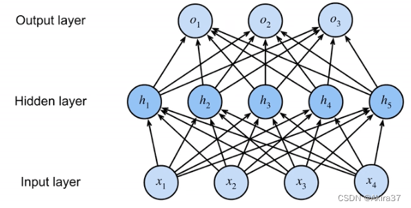

net = nn.Sequential(nn.Flatten(),
                    nn.Linear(784, 256),
                    nn.ReLU(),
                    nn.Linear(256, 10))

def init_weights(m):
    if type(m) == nn.Linear:
        nn.init.normal_(m.weight, std=0.01)

net.apply(init_weight)

4.2 常见激活函数

激活函数（Activation Function）：在仿射变换之后对每个隐藏单元应用的函数，大多数都是非线性的，其输出被称为活性值（Activations）。用于发挥多层架构的潜力，防止将多层感知机退化成线性模型。

4.2.1 ReLU

修正线性单元（Rectified Linear Unit，ReLU）：仅保留正元素并丢弃所有负元素

\begin{aligned}
\text{ReLU}(x)=\max(0,x)
\end{aligned}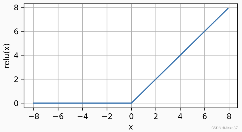

导数（x=0时不可导，此时常默认使用左导数）：

\begin{aligned}
\frac{\mathrm{d}}{\mathrm{d}x}\text{ReLU}(x)=\begin{cases}
 0, &x<0 \\
 1, &x>0
\end{cases}
\end{aligned}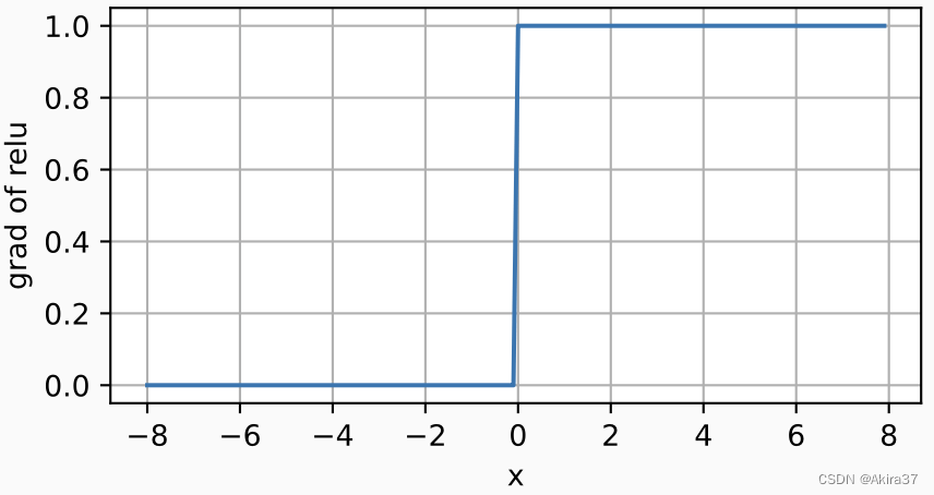

变体——参数化ReLU（Parameterized ReLU，pReLU）：为ReLU添加了一个线性项，即使参数是负的，某些信息仍可以通过

\begin{aligned}
\text{pReLU}(x)=\max(0,x)+\alpha \min(0,x)
\end{aligned}

4.2.2 Sigmoid

Sigmoid函数：输入压缩到区间(0, 1)中的某个值，因此通常称为挤压函数（squashing function）

\begin{aligned}
\text{sigmoid}(x)=\frac1{1+\exp(-x)}
\end{aligned}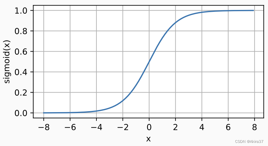

导数：

\begin{aligned}
\frac{\mathrm{d}}{\mathrm{d}x}\text{sigmoid}(x) &=\frac{\exp(-x)}{(1+\exp(-x))^2}\\
 &=\text{sigmoid}(x)(1-\text{sigmoid}(x))
\end{aligned}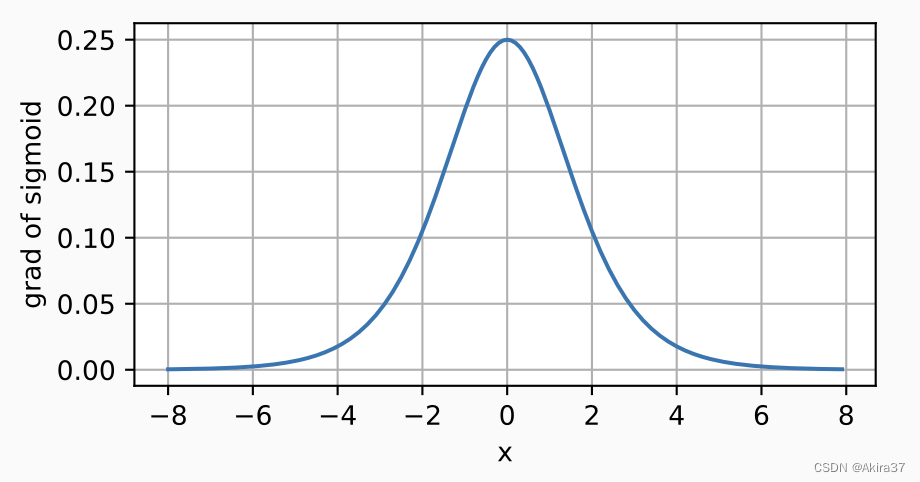

4.2.3 tanh

双曲正切函数（tanh）：将输入压缩转换到区间(-1, 1)上

\begin{aligned}
\tanh(x)=\frac{1-\exp(-2x)}{1+\exp(-2x)}
\end{aligned}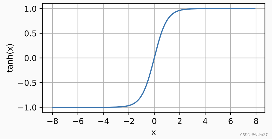

导数：

\begin{aligned}
\frac{\mathrm{d}}{\mathrm{d}x}\tanh(x)=1-\tanh^2(x)
\end{aligned}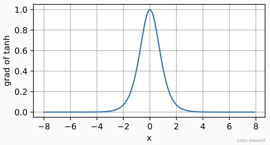

4.3 模型选择、欠拟合和过拟合

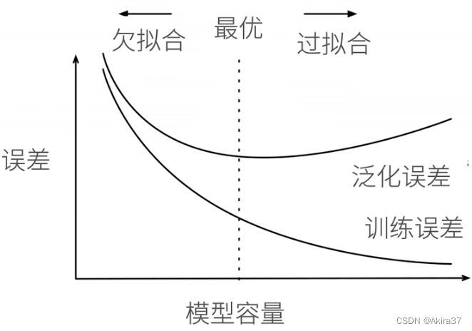
训练误差（Training Error）：模型在训练数据上的误差
泛化误差（Generalization Error）：模型在新数据上的误差

验证数据集（Validation Dataset）：用来评估模型好坏的数据集（不应跟训练数据混在一起）
测试数据集（Test Dataset）：只用一次的数据集

K折交叉验证：在没有足够多数据时使用。将训练数据分割成K块；执行K次模型训练与验证，每轮迭代使用其中1块作为验证数据集，其余的作为训练数据；最后报告K个验证集误差的平均值。常取K=5或10

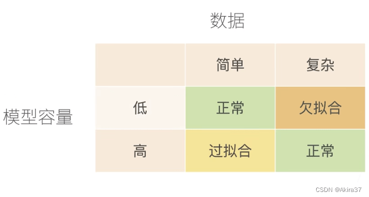
模型容量（模型复杂性）：拟合各种函数的能力，需要匹配数据复杂度（取决于多个重要因素——样本个数、每个样本的元素个数、时间/空间结构、多样性）。

• 低容量的模型难以拟合训练数据——欠拟合（Underfitting）
• 高容量的模型可以记住所有的训练数据——过拟合（Overfitting）。

VC维：统计学习理论的一个核心思想。对于一个分类模型，VC等于一个最大的数据集的大小，不管如何给定标号，都存在一个模型来对它进行完美分类。
【例】2维输入的感知机，VC维=3 —— 能够分类任何3个点，但不是4个（xor）。如下图所示

支持N维输入的感知机的VC维为N+ 1
一些多层感知机的VC维O(N\log_2 N)
在深度学习中很少使用，因为衡量不是很准确，且计算深度学习模型的VC维很困难

4.4 权重衰退（L2正则化）

权重衰退/L_2正则化（Weight Decay）是最广泛使用的正则化的技术之一，通过L_2正则项使得模型参数不会过大，从而控制模型复杂度。

硬性限制：直接限制参数值的选择范围\theta来控制模型容量（通常没必要限制偏移b），越小的\theta意味着更强的正则项，即

\begin{aligned}
\min L(\mathbf{w},b)\ \text{ subject to }\ \lVert \mathbf{w} \rVert ^2≤\theta
\end{aligned}

柔性限制：在上式的基础上，对每个\theta，都可以找到正则化常数\lambda，控制L_2正则项\lVert \mathbf{w} \rVert^2的重要程度：\lambda=0时无作用；\lambda \rightarrow \infin时\mathbf{w}^* \rightarrow \mathbf{0}。即使用验证数据拟合L(\mathbf{w},b) + \frac \lambda 2 \lVert \mathbf{w} \rVert ^2。

根据此柔性限制进行梯度下降、更新权重（通常\eta \lambda<1）：

\begin{aligned}
\frac{\partial }{\partial \mathbf{w} }\left(l(\mathbf{w},b)+\frac \lambda 2 \lVert \mathbf{w} \rVert ^2\right)=\frac{\partial l(\mathbf{w},b)}{\partial \mathbf{w}}+\lambda\mathbf{w}
\end{aligned}

\begin{aligned}
\mathbf{w} &\leftarrow \mathbf{w}-\eta \frac{\partial }{\partial \mathbf{w} }\left(l(\mathbf{w},b)+\frac \lambda 2 \lVert \mathbf{w} \rVert ^2\right)\\
 &= (1-\eta \lambda)\mathbf{w}-\eta \frac{\partial l(\mathbf{w},b)}{\partial \mathbf{w}}
\end{aligned}

4.5 丢弃法（Dropout）

丟弃法/暂退法（Dropout）：在层之间加入噪音，根据超参数丢弃概率p（常取0.5, 0.9, ...）将一些输出项随机置来控制模型复杂度。若对 \mathbf{x}加入噪音得到\mathbf{x'}，期望E[\mathbf{x'}]=\mathbf{x}，则对每个元素进行如下扰动

\begin{aligned}
x_i'=\text{dropout}(x_i)=\begin{cases}
 0, & \text{with probability } p \\
 \frac{x_i}{1-p}, & \text{otherwise}
\end{cases}
\end{aligned}

通常将丟弃法作用在隐藏全连接层的输出上

\begin{aligned}
\mathbf{h}&=\sigma(\mathbf{W}_1\mathbf{x}+\mathbf{b_1})   \\
\mathbf{h'} &= \text{dropout}(\mathbf{h})\\
 \mathbf{o} &=\mathbf{W}_2\mathbf{h'}+\mathbf{b_2} \\
\mathbf{y} &= \text{softmax}(\mathbf{o} )
\end{aligned}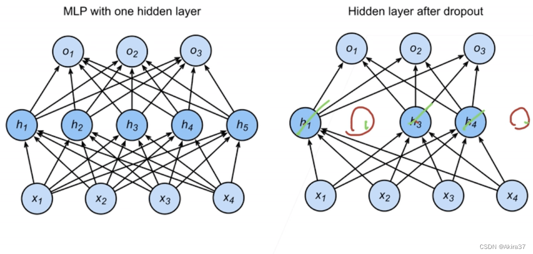

dropout是正则项，只在训练中使用，影响模型参数的更新。在推理过程中，dropout直接返回输入，这样也能保证确定性的输出，即

 \mathbf{h} = \text{dropout}(\mathbf{h})

PyTorch实现：

nn.Dropout(p)   # p：丢弃概率

net = nn.Sequential(
    nn.Flatten(),
    nn.Linear(784, 256),
    nn.ReLU(),
    # 在第一个全连接层之后添加一个dropout层
    nn.Dropout(dropout1),
    nn.Linear(256, 256),
    nn.ReLU(),
    # 在第二个全连接层之后添加一个dropout层
    nn.Dropout(dropout2),
    nn.Linear(256, 10)
)

4.6 数值稳定性与模型初始化

设一个深度神经网络（Dense/Deep Neural Network，DNN）具有L层，输入为 \mathbf{x}，输出为\mathbf{o}，第l层由权重为\mathbf{W}^{(l)}、隐藏变量为\mathbf{h}^{(l)}的变换f_l定义（令\mathbf{h}^{(0)}=\mathbf{x}），则可表示为

\begin{aligned}
\mathbf{h}^{(l)}=f_l(\mathbf{h}^{(l-1)}) \text{ hence } \mathbf{o}=f_L \circ f_{L-1} \circ \cdots \circ f_1(\mathbf{x})
\end{aligned}

若所有隐藏变量和输入都是向量， 则可将输出\mathbf{o}关于任意一组参数\mathbf{W}^{(l)}的梯度表示为

\begin{aligned}
\partial_{\mathbf{W}^{(l)}}\mathbf{o}=\partial_{\mathbf{h}^{(L-1)}}\mathbf{h}^{(L)} \partial_{\mathbf{h}^{(L-2)}}\mathbf{h}^{(L-1)} \cdots \partial_{\mathbf{h}^{(l+1)}}\mathbf{h}^{(l+2)}  \partial_{\mathbf{h}^{(l)}}\mathbf{h}^{(l+1)} \partial_{\mathbf{W}^{(l)}}\mathbf{h}^{(l)}
\end{aligned}

由上式易知，深度神经网络的梯度是L-l个矩阵与1个梯度向量的乘积，如此多项的乘积可能非常大，也可能非常小，使得出现不稳定梯度，极易产生以下两种数值稳定性问题：

• 梯度爆炸（Gradient Exploding）：参数更新过大，破坏了模型的稳定收敛

  • 值超出值域：对于16位浮点数尤为严重（数值区间6e-5~6e4）
  • 对学习率敏感，可能需在训练过程中不断调整学习率
    • 学习率太大→大参数值→更大的梯度
    • 学习率太小→训练无进展

• 梯度消失（Gradient Vanishing）： 参数更新过小，在每次更新时几乎不会移动，导致模型无法学习

  • 梯度值变成0：对16位浮点数尤为严重
  • 训练没有进展，不管如何选择学习率
  • 对于底部层尤为严重：仅仅顶部层训练的较好，无法让神经网络更深

让训练更加稳定：

1. 让梯度值在合理的范围内。（例如在[1e-6, 1e3]上）
2. 将乘法变加法（ResNet、LSTM）
3. 归一化（梯度归一化、梯度裁剪）
4. 合理的权重初始和激活函数
   • 让每层的方差是一个常数：将每层的输出和梯度都看做随机变量，让它们的均值和方差都保持一致

解决（或至少减轻）数值稳定性问题的一种方法是进行合理的参数初始化。通常可用正态分布初始化权重，或直接使用框架默认的随机初始化方法。（参考前述各种网络模型）

Xavier初始化：对于没有非线性的全连接层（如隐藏层），其共有n_\text{in}个输入、n_\text{out}个输出，第j个输入x_j的权重为w_{ij}，则第i个输出o_i可表示为

\begin{aligned}
o_i=\sum_{j=1}^{n_\text{in}}w_{ij}x_j
\end{aligned}

假设权重w_{ij}从均值为、方差为\sigma^2的同一分布中独立抽取，输入层全体x_j也满足均值为、方差为\gamma^2且与w_{ij}彼此独立，则可计算得o_i的均值和方差为

\begin{aligned}
E[o_i] &=\sum_{j=1}^{n_\text{in}}E[w_{ij}x_j]\\
&=\sum_{j=1}^{n_\text{in}}E[w_{ij}]E[x_j]\\
&=0\\
\text{Var}[o_i] &=E[o_i^2]-E^2[o_i]\\
&=\sum_{j=1}^{n_\text{in}}E[w_{ij}^2x_j^2]-0\\
&=\sum_{j=1}^{n_\text{in}}E[w_{ij}^2]E[x_j^2]\\
&=n_\text{in}\sigma^2\gamma^2
\end{aligned}

要想保持方差始终为\gamma^2不变，需设置n_\text{in}\sigma^2=1。反向传播同理，参考上述前向传播的推断过程可知需设置 n_\text{out}\sigma^2=1。显然无法同时满足这两个条件。Xavier初始化只需满足以下条件：

\begin{aligned}
\frac12(n_\text{in}+n_\text{out})\sigma^2=1 \Leftrightarrow \sigma=\sqrt{\frac2{n_\text{in}+n_\text{out}}}
\end{aligned}

通常Xavier初始化从均值为0、方差为\sigma^2=\frac2{n_\text{in}+n_\text{out}}的高斯分布中采样权重。也可以改为选择从均匀分布中抽取权重时的方差，由均匀分布U(-a,a)的方差为\frac{a^3}3，代入上式可得Xavier初始化值域为

\begin{aligned}
U(-\sqrt{\frac6{n_\text{in}+n_\text{out}}},\sqrt{\frac6{n_\text{in}+n_\text{out}}})
\end{aligned}

---

5 优化算法

本章是对3.3“解析解”结尾求解方法的扩充，详细介绍各类重要的优化算法。

5.1 优化基础知识

在优化中，损失函数通常被称为优化问题的目标函数，且大多数优化算法都关注的是最小化（若要最大化，只需给目标函数加负号）。对于目标函数f:\mathbb{R}^n \rightarrow \mathbb{R}，其优化的一般形式为

\begin{aligned}
\text{minimize } f(\mathbf{x}) \text{ subject to } \mathbf{x}\in \mathcal{X}
\end{aligned}

若\mathcal{X}=\mathbb{R}^n则为不受限，否则为限制集合，例如

\begin{aligned}
\mathcal{X}=\{ \mathbf{x}\mid h_1(\mathbf{x})=0, \dots,h_m(\mathbf{x})=0,g_1(\mathbf{x})≤0,\dots,g_r(\mathbf{x})≤0 \}
\end{aligned}

5.1.1 优化常见问题

全局最小值vs局部最小值

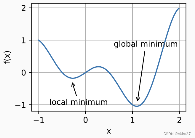
全局最小值（Global Minimum）：在x处对应的f(x)值是整个域\mathcal{X}中目标函数的最小值，则f(x)就是全局最小值。即存在\mathbf{x}^*满足

\begin{aligned}
\forall\ \mathbf{x}\in \mathcal{X},\ f(\mathbf{x}^*)≤f(\mathbf{x})
\end{aligned}

局部最小值（Local Minimum）：在x处对应的f(x)值小于在x附近任意其他点的f(x)值，则f(x)可能是局部最小值。即存在\mathbf{x}^*满足

\begin{aligned}
\exists\ \epsilon,\ \forall\ \mathbf{x}:\lVert \mathbf{x} -\mathbf{x}^* \rVert ≤ \epsilon,\ f(\mathbf{x}^*)≤f(\mathbf{x})
\end{aligned}

使用迭代优化算法来求解，一般只能保证找到局部最小值。通过最终迭代获得的数值解可能仅使目标函数局部最优，而不是全局最优。

其他问题

鞍点（Saddle Point）是指函数的所有梯度都消失但既不是全局最小值也不是局部最小值的任何位置。

梯度消失（Gradient Vanishing）：见4.6“数值稳定性与模型初始化”。

5.1.2 凸性

凸性（Convexity）在优化算法的设计中起到至关重要的作用。（注意此处的“凸”指的是“向下凸”！）

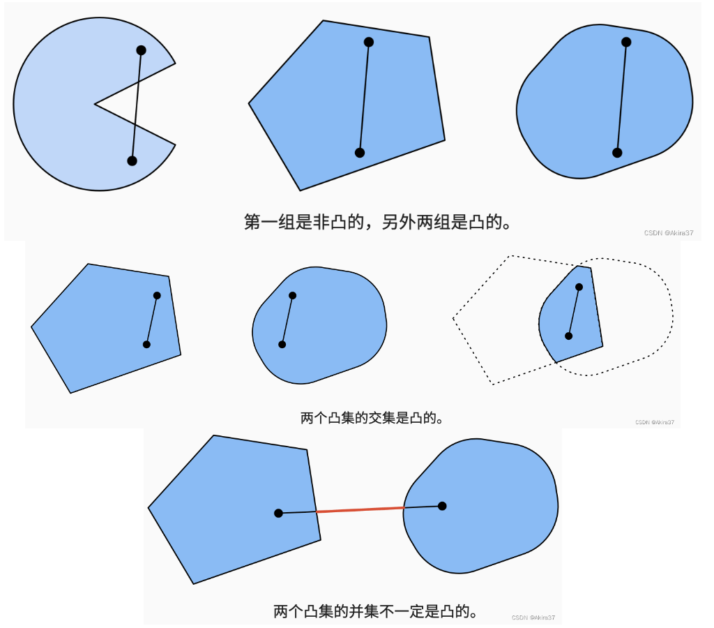
凸集（Convex Set）：若对于任何a,b \in\mathcal{X}，连接a和b的线段也位于\mathcal{X}中，则称该向量空间中的集合\mathcal{X}是凸（Convex）的，即

\begin{aligned}
\forall\ \lambda \in [0,1],\ \forall\ a,b \in \mathcal{X},\  \lambda a+(1-\lambda)b \in \mathcal{X}
\end{aligned}

若\mathcal{X}和\mathcal{Y}是凸集，则\mathcal{X}\cap \mathcal{Y}也是凸集。反之不成立。对于并集也不成立。

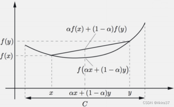
凸函数（Convex Function）：给定一个凸集\mathcal{X}，若函数f:\mathcal{X}\rightarrow \mathbb{R}是凸的，则

\begin{aligned}
\forall\ \lambda \in [0,1],\ \forall\ x,x' \in \mathcal{X},\ \lambda f(x)+(1-\lambda)f(x')≥f(\lambda x+(1-\lambda)x;)
\end{aligned}

若x≠x',\ \lambda\in (0,1)是、时不等式严格成立，则称为严格凸函数。

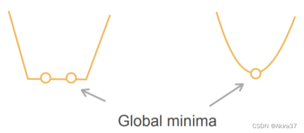
• 如果目标函数f是凸的，且限制集合\mathcal{X}也是凸的，则为凸优化问题，那么局部最小一定是全局最小。
• 严格凸优化问题有唯一的全局最小。

典例：

• 凸：
  1. 线性回归f(\mathbf{x})=\lVert \mathbf{Wx}-\mathbf{b} \rVert^2
  2. Softmax回归
• 非凸（大多数）：MLP、CNN、RNN、注意力……

5.2 梯度下降

梯度下降（Gradient Descent）是最简单的迭代求解算法。设目标函数为f(\mathbf{x})，随时间增加执行以下操作

\begin{aligned}
\mathbf{x}\leftarrow \mathbf{x}-\eta \nabla f(\mathbf{x})
\end{aligned}

其中\eta称为学习率（Learning Rate）。

5.3 随机梯度下降

随机梯度下降（Stochastic Gradient Descent，SGD）：给定n个样本的训练数据集，设f_i(\mathbf{x})是关于索引i的训练样本的损失函数，则目标函数f(\mathbf{x})=\frac1n \sum\limits_{i=1}^n f_i(\mathbf{x})，梯度\nabla f(\mathbf{x})=\frac1n \sum\limits_{i=1}^n \nabla f_i(\mathbf{x})。计算该导数开销太大，因此改用SGD来不断逼近目标，即

\begin{aligned}
\mathbf{x}\leftarrow \mathbf{x}-\eta \nabla f_i(\mathbf{x}),\ i=1,2,\dots,n
\end{aligned}

易知随机梯度\nabla f_i(\mathbf{x})是对完整梯度\nabla f(\mathbf{x})的无偏近似（期望一样），即

\begin{aligned}
E_i[\nabla f_i(\mathbf{x})] &=\frac1n \sum_{i=1}^n \nabla f_i(\mathbf{x})\\
 &=\nabla f(\mathbf{x})
\end{aligned}

5.4 小批量梯度下降

小批量随机梯度下降（Minibatch Gradient Descent）：最常用的优化算法。对梯度下降和随机梯度下降的折中，取一个小批量\mathcal{B}来执行上述操作，提高计算效率。即

\begin{aligned}
\mathbf{x}\leftarrow \mathbf{x}-\frac{\eta}{|\mathcal{B}|}\sum_{i\in \mathcal{B}} \nabla f_i(\mathbf{x})
\end{aligned}

与随机梯度下降一样，也是无偏近似。并且方差显著降低：由于小批量梯度由正在被平均计算的|\mathcal{B}|个独立梯度组成，其标准差降低了|\mathcal{B}|^{-\frac12}。

5.5 冲量法

冲量法为了能够从小批量梯度下降方差减少的影响中受益，甚至超过小批量上的梯度平均值，使用泄漏平均值（Leaky Average）取代梯度计算。今后使用参数更新的另一种记法：设时间为t，则冲量法更新\mathbf{w}的过程为

\begin{aligned}
\mathbf{g}_t &:= \frac{1}{|\mathcal{B}|}\sum\limits_{i\in \mathcal{B}}\nabla f_i(\mathbf{x_{t-1}})\\
\mathbf{v}_t &=\beta \mathbf{v}_{t-1}+\mathbf{g}_t\\
\mathbf{w}_t &=\mathbf{w}_{t-1}-\eta \mathbf{v}_t
\end{aligned}

其中\beta\in (0,1)，常取0.5,0.9,0.95,0.99。\mathbf{v}称为冲量（Momentum），其梯度平滑，可展开为

\mathbf{v}_t=\mathbf{g}_t+\beta g_{t-1}+\beta^2 \mathbf{g}_{t-2}+ \beta^3 \mathbf{g}_{t-3}+\cdots

5.6 Adam

Adam算法将上述所有高级算法技术汇总到一个高效的学习算法中。其关键是对梯度做平滑，且对梯度各个维度值做重新修正。使用状态变量

\begin{aligned}
\mathbf{v}_t &=\beta_1\mathbf{v}_{t-1}+(1-\beta_1)\mathbf{g}_t\\
\mathbf{s}_t &=\beta_2\mathbf{s}_{t-1}+(1-\beta_2)\mathbf{g}_t^2
\end{aligned}

常设置非负加权参数\beta_1=0.9,\beta_2=0.999。根据上述冲量法中的冲量展开式知，梯度依旧平滑。由\mathbf{v}_0=\mathbf{s}_0=\mathbf{0}，为避免初始偏差过大，根据\sum\limits_{i=0}^t \beta^i=\frac{1-\beta^t}{1-\beta}修正\mathbf{v},\ \mathbf{s}为

\begin{aligned}
\mathbf{\hat v}_t &=\frac{\mathbf{v}_t}{1-\beta_1^t}\\
\mathbf{\hat s}_t &=\frac{\mathbf{s}_t}{1-\beta_2^t}
\end{aligned}

计算修正后的梯度为

\begin{aligned}
\mathbf{g}'_t=\frac{\eta \mathbf{\hat v}_t}{\sqrt{\mathbf{\hat s}_t}+\epsilon}
\end{aligned}

为了在数值稳定性和逼真度之间取得良好的平衡，常选择\epsilon=10^{-6}。最后进行简单更新

\begin{aligned}
\mathbf{w}_t=\mathbf{w}_{t-1}-\eta \mathbf{g}'_t
\end{aligned}

---

6 PyTorch深度学习计算

本节介绍PyTorch中如何具体实现前述的各项技术。

6.1 层和块

一个块可以由许多层或块组成。块可以包含代码，负责大量的内部处理，包括参数初始化和反向传播。层和块的顺序连接可以由Sequential块处理。

import torch
import torch.nn.functional as F
from torch import nn

class MLP(nn.Module):
    def __init__(self):
        super().__init__()
        self.net = nn.Sequential(nn.Linear(20, 64), nn.ReLU(),
                                 nn.Linear(64, 32), nn.ReLU())
        self.linear = nn.Linear(32, 16)

    def forward(self, X):
        return self.linear(self.net(X))

net = MLP()
y_hat = net(X)

6.2 参数管理

Sequential内部组织

6.2.1 参数访问

直接打印可得Sequential类的内部组织：

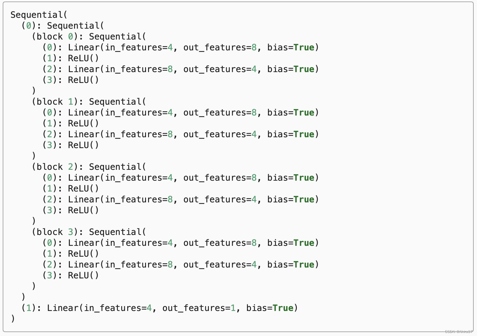
Sequential类相当于列表，可以直接用索引访问对应的层。对于嵌套块，因为层是分层嵌套的，所以也可以像通过嵌套列表索引一样访问它们。相关方法和成员参见前文。

# 获取参数的名称及其值的字典
net[2].state_dict()         # 返回OrderedDict类型

# 访问参数及其成员
net[2].bias                 # 获取偏移（包含值和其他信息）
rgnet[0][1][0].bias.data    # 获取偏移的值
net[2].weight.grad          # 获取权值的梯度

# 一次性访问所有参数
[(name, param.shape) for name, param in net[0].named_parameters()]  # 访问0号层的所有参数
[(name, param.shape) for name, param in net.named_parameters()]     # 访问整个网络所有层的所有参数

6.2.2 参数初始化

默认情况下，PyTorch会根据一个范围均匀地初始化权重和偏置矩阵， 这个范围是根据输入和输出维度计算出的。

1. 内置初始化：调用PyTorch的nn.init模块提供的初始化函数

# 初始化为标准正态分布
def init_normal(m):
    if type(m) == nn.Linear:
        nn.init.normal_(m.weight, mean=0, std=0.01)
        nn.init.zeros_(m.bias)

net.apply(init_normal)

# 初始化为常数1
def init_constant(m):
    if type(m) == nn.Linear:
        nn.init.constant_(m.weight, 1)
        nn.init.zeros_(m.bias)

net.apply(init_constant)

# 对不同块应用不同的初始化方法：对0号层用Xavier初始化，对2号层初始化为常数42
def init_xavier(m):
    if type(m) == nn.Linear:
        nn.init.xavier_uniform_(m.weight)

def init_42(m):
    if type(m) == nn.Linear:
        nn.init.constant_(m.weight, 42)

net[0].apply(init_xavier)
net[2].apply(init_42)

2. 自定义初始化：当深度学习框架没有提供实际需要的初始化方法时可自定义初始化方法。
   【例】使用以下的分布为任意权重参数w定义初始化方法

w\sim \begin{cases}
 U(5,10) & \text{ with probability } \frac14 \\
 0 & \text{ with probability } \frac12 \\
 U(-10,-5) & \text{ with probability } \frac14
\end{cases}

# 自定义初始化
def my_init(m):
    if type(m) == nn.Linear:
        print("Init", *[(name, param.shape)
                        for name, param in m.named_parameters()][0])
        nn.init.uniform_(m.weight, -10, 10)
        m.weight.data *= m.weight.data.abs() >= 5

net.apply(my_init)

3. 直接初始化！

net[0].weight.data[:] += 1
net[0].weight.data[0, 0] = 42
net[0].weight.data[0]

6.2.3 参数绑定

在Sequential外定义共享层变量，在Sequential中的多个层间共享参数

shared = nn.Linear(8, 8)
net = nn.Sequential(nn.Linear(4, 8), nn.ReLU(),
                    shared, nn.ReLU(),
                    shared, nn.ReLU(),
                    nn.Linear(8, 1))

6.3 自定义层

有时会遇到或要自己发明一个现在在深度学习框架中还不存在的层。 在这些情况下，必须构建自定义层。可以将自定义层像预置层一样作为组件合并到更复杂的模型中。

构造不带参数的层：

class CenteredLayer(nn.Module):
    """从其输入中减去均值的层"""
    def __init__(self):
        super().__init__()

    def forward(self, X):
        return X - X.mean()

layer = CenteredLayer()
net = nn.Sequential(nn.Linear(8, 128), CenteredLayer())

构建带参数的层：

class MyLinear(nn.Module):
    """自定义版的全连接层"""
    def __init__(self, in_units, units):
        super().__init__()
        self.weight = nn.Parameter(torch.randn(in_units, units))
        self.bias = nn.Parameter(torch.randn(units,))

    def forward(self, X):
        linear = torch.matmul(X, self.weight.data) + self.bias.data
        return F.relu(linear)

linear = MyLinear(5, 3)
net = nn.Sequential(MyLinear(64, 8), MyLinear(8, 1))

6.4 读写文件

加载和保存张量

x = torch.arange(4)
y = torch.zeros(4)
mydict = {'x': x, 'y': y}

# 保存或读取张量
torch.save(x, 'x-file')
x2 = torch.load('x-file')

# 保存或读取张量列表
torch.save([x, y], 'x-files')
x2, y2 = torch.load('x-files')

# 保存或读取从字符串映射到张量的字典
torch.save(mydict, 'mydict')
mydict2 = torch.load('mydict')

加载和保存模型参数

net = MLP()     # 5.1的MLP网络

# 存储网络：存参数的字典
torch.save(net.state_dict(), 'mlp.params')
# 读取网络（需先定义相同类的网络）
clone = MLP()
clone.load_state_dict(torch.load('mlp.params'))